SIMPLE OBSERVATIONS OF 21 CM HYDROGEN LINE EMISSION

An earlier version of the article presented here appeared in the Australian Journal of Astronomy, vol 5 issue 4 (1994), pp 121-133.

HYDROGEN-LINE OBSERVATIONS OF THE GALAXY AND THE MAGELLANIC CLOUDS by Mal Wilkinson and John Kennewell

A series of observations of the radio emission from atomic hydrogen in the spiral arms of our Galaxy and in the neighbouring Magellanic Clouds has been conducted using relatively simple observing equipment. Accurate measurements of the intensity and Doppler shift of this emission with respect to the hydrogen line rest frequency (1420.406 MHz) were made at a number of galactic longitudes. From these observations, the relative velocity of the regions under observation with respect to Earth and the local standard of rest (LST) could be determined. Some interesting conclusions can be drawn about the structure and velocity distribution of hydrogen within our Galaxy.

1 INTRODUCTION

The study of astronomy and the exploration of space have given us an ever expanding perspective on our position in the Universe in which we live. In historic times, Earth was seen as the centre of the Universe, an idea which seemed consistent with religious teachings which saw humankind as God's principal creation.

Nicolaus Copernicus, himself a man of religion, was the first to convincingly deny Earth such a central place in the cosmos. In his mammoth work De revolutionibus orbium coelestium libri VI (Six books on the revolutions of the celestial spheres) published in 1543, he placed the Sun firmly at the centre of the Solar System.

On 14 Feb 1990, 13 years after launch, and nearly 450 years after Copernicus, the robotic explorer of deep space, Voyager 1, from a position nearly 6 billion kilometres from the Sun and 32° above the ecliptic, turned its cameras earthward and photographed the Solar System from space for the first time. From this position. Earth was a mere 0.12 pixel on the CCD photographic image. Even the mighty Sun was only one fortieth the size as seen from Earth.

Such is the vastness of space however, that to gain a similar perspective of our Galaxy and the Sun's position within it, would take no less than 300 million years, if we (travelled at a velocity of 60,000 km/h, the same velocity with which Voyager 1 left our Solar System forever. Even travelling at the speed of light it would take almost 9,000 years!

It is not surprising then, that astronomers have searched for over 250 years, since the time of William Herschel, for indirect ways to understand what our Galaxy would look like from a position in space well above the galactic plane. Only relatively recently has it become possible to fill in the picture, not so much by studying the visible stars, but rather the invisible hydrogen gas between the stars. Interstellar atomic hydrogen is an important component of the structure of our Galaxy, forming a large flattened disc 100 to 300 parsecs thick which shows internal spiral arm structure similar to that of the visible stars.

The ground state of this hydrogen can assume two different energy levels (figure 1), related to whether the proton and electron magnetic moments are parallel (high energy) or anti-parallel (low energy). When transitions occur between these two states as a result of random collisions between atoms, a photon of radio energy is emitted or absorbed at a frequency of 1420.406 MHz (more precisely 1,420,405,751.786 Hz).

Figure 1. Generation mechanism for the hydrogen line emission. The proton and electron, which make up the hydrogen atom, can be considered to have spin and an associated magnetic field and magnetic moment (indicated by the large arrows). When these moments are parallel (left) the atom is in a high energy state whereas when they are antiparallel (right) the atom is in a lower energy state. It is the transistion between these two energy states which results in the generation of radio emission at the hydrogen line frequency of 1420.406 MHz.

By analogy with emission lines in visible spectra, this is referred to as hydrogen line emission. Although the probability of these energy transitions is very small - only one transition occurs every hundred years or so - there is sufficient hydrogen in the galaxy so that the combined effect of all these transitions produces weak radio emission which is detectable with a suitable radio telescope.

The presence of hydrogen line emission was theoretically predicted by Hendrick C. van de Hulst of the University of Leiden Observatory in 1944 April. A race then developed between Dutch and American radio astronomers to detect the line. This was no easy task since it required the construction of extremely sensitive equipment. The race was finally won by Harold Ewen of Harvard University who detected the line early in the morning of 25 March 1951. Within weeks however, the Dutch group, led by Jan Oort was also successful, despite a major setback during which their receiving equipment was destroyed by a mysterious fire. Realizing the importance of this discovery, Australian radio astronomers led by Joe Pawsey of the CSIRO rapidly assembled a makeshift receiver and confirmed the American and Dutch results in July 1951.

When the hydrogen is in relative motion with respect to the line of sight to the observer, the line emission is observed at a frequency which is Doppler-shifted above or below the rest frequency of 1420.406 MHz depending upon whether the emitter is moving respectively towards or away from the observer. Since this frequency shift is easily measured, the relative velocity of the observed hydrogen can be calculated. It is this feature which makes hydrogen line emission such a useful tool in the study of galactic dynamics.

Another reason for the importance of hydrogen line measurements is that since the wavelength of the emission is much longer than that of visible light, it is unaffected by the dust clouds which exist in the plane of the Galaxy. Because this dust effectively obscures starlight, early visual studies of galactic structure were limited to a region within a few kiloparsecs of the Sun. When radio techniques were introduced they were spectacularly successful in identifying spiral arm structure right across the Galaxy.

Where hydrogen line emission is being received simultaneously from several hydrogen clouds in different spiral arms of the Galaxy, all with different relative motions with respect to the observer, the received signal may contain a range of Doppler-shifted frequencies and hence the radio spectrum becomes very complex. Nevertheless, astronomers have developed modelling techniques to unravel these data to provide a wonderfully detailed map of the spiral structure of our Galaxy.

Studies of the hydrogen line emission have revolutionized our knowledge of the structure of our own Galaxy and galaxies beyond, and have contributed to the current debate on dark matter. It is worth remembering, that as late as 1920, our knowledge of galactic structure and distances was so limited, that astronomers of the calibre of Shapley and Curtis were debating whether the spiral 'nebulae', such as the great spiral galaxy in Andromeda, were part of our own Galaxy or external to it!

2 INTO PRACTICE

Published data on the intensity of hydrogen line emission from the galactic plane suggest a maximum equivalent black body temperature of around 100 K or less can be expected depending upon the equivalent optical depth of the emitting cloud. If this emission is present over a sufficiently-large angular extent to fill the beam of a moderately-directive antenna, then this is the temperature that the antenna radiation resistance would assume. For emission from hydrogen gas in the local arm, this condition is approximately satisfied.

Modern GAsFET pre amplifiers for 1420 MHz have equivalent noise temperatures of near 100 K, and allowing for some further contributions from antenna spillover, transmission line losses and the receiver itself totalling 100 K gives a system noise temperature of 200 K. Hence, neglecting the background temperature, an antenna temperature of 100 K on the line should give a measurable noise power increase of around 50%. This increase should be easily detectable. With a small integration time of around five seconds much smaller changes can be detected.

For detecting emission from spiral arms only a few kiloparsecs away from the Sun, the situation is more difficult. Assuming that the thickness of the galactic hydrogen disc is 300 parsecs, an antenna beamwidth of around 5° is required to achieve an antenna temperature of 100 K from clouds at a distance of three kiloparsecs, since these clouds subtend an angle of 5° at the observer. The antenna temperature may be significantly less than this if the cloud is optically thin or the assumed thickness is less than 300 parsecs.

Therefore, using available technology, a 5° antenna beamwidth is probably the minimum requirement for useful hydrogen line observations and leads to a required antenna diameter of 14 wavelengths or around three metres. A beamwidth of less than 1° would be desirable for studies which include the galactic centre or spiral structure across the Galaxy.

Extragalactic objects such as the Magellanic Clouds, whose hydrogen clouds are of significant angular extent despite their large distances, should also be detectable with moderate-sized antennas. Some of these predictions will be tested in the observations which follow.

3 TELESCOPE CONSTRUCTION

3.1 Receiving Equipment

The configuration employed to make the observations is illustrated in figure 2. The MITEQ/AFD2 low noise GAsGET 1-2 GHz preamplifier and the AR3000 scanning receiver are commercially available equipment. The AR3000 was powered by a regulated battery power supply. A GAsFET switch was constructed using an ANZAC SW-239 RF switch. The measured insertion loss for this switch, including RF connectors, was 0.6 dB at 1420.406 MHz.

Figure 2. Basic radio telescope used for hydrogen line observations.

The receiver was used in AM mode with a 6 dB bandwidth of 12 kHz. The stability of the noise output from the AR3000 was checked prior to observing by tuning over a range of frequencies with the receiver antenna connected to a 50 ohm termination. The noise output for this test and during the observations was measured using a Fluke model 8020A AC digital voltmeter which was internally modified to increase the integration time to five seconds.

A knowledge of scanner performance while recording noise over a range of frequencies was important to the success of the project. The output varied periodically with frequency (figure 3) but it was possible to minimise this source of variation by experimentally selecting an appropriate frequency increment - in this case 50 kHz. One spurious response (birdie) was noted within the hydrogran line frequency range, but this frequency could be avoided by using memory programmed frequency tuning points during observations.

Figure 3. The variation in mean noise output when the scanner antenna input was terminated in 50 ohms and the scanner was tuned in 10 kHz steps.

The frequency calibration accuracy of the AR3000 at 1420 MHz was found to be excellent and was within 1 kHz of the indicated value.

The noise output level of the receiver/preamp combination was quite sensitive to ambient temperature changes. To minimise these effects, the measurements were made after several hours warm up and generally late in the evening when temperatures were stable. In addition, a system noise calibration was performed immediately after each profile observation. These were done using a specially designed dual-heated load calibration technique in which the receiving system was switched between two 50 ohm terminations, one of which was heated by a known amount (usually 40° C) with respect to the other.

Details of the electronics for the dual heated load calibrator are shown in figure 4. Fifty-ohm termination resistor R2 was heated to a known temperature difference with respect to Rl. This difference was used to calibrate the radio telescope. The temperature of each termination was measured using a temperature to current converter. These (opposite polarity) currents were compared via amplifier IC1 and comparator IC2, to an offset current proportional to the required temperature difference. This was provided through SW1-SW5 (each giving either a 10 K or a 2 K step) and a set of resistors. A servo loop, which included an optical isolator and a three-transistor heater arrangement TRl,2,3 were used to control the temperature of R2. Fifty-ohn load R2, the temperature to current sensor, and the heater transistors were embedded in a 50-g block of aluminium which acted as a thermal mass (probe T_Heat). Similarly for Rl except there was no heater (probe T_Amb).

Figure 4. Circuit for the dual heated load calibrator.

3.2 Antenna Construction

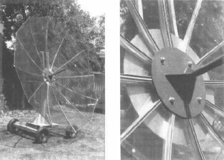
A parabolic antenna with a diameter of three metres, complete with mounting, can occupy a considerable area in a suburban back garden, so right from the outset a four quadrant (quarter circle) design evolved so that the parabola could be disassembled into four pieces after each observing session. Each section is light in weight to facilitate assembly, disassembly and storage when not in use, by one person. Since the antenna is not at the mercy of the elements, the ability to resist high wind loads is unnecessary so that cost and weight can be reduced.

The ribs were fabricated using a novel dual pre-stressed truss technique. The rear truss was made from 12.5 x 1-mm square tubular aluminium which was bent by hand in a vice in three places. The position of these bends was calculated (1)to conform to a segmented approximation of a parabola and (2)so that each bend had the same included angle, thus facilitating construction. A smaller section of 10 x 1 mm U-shaped aluminium of the type used in aluminium fly-wire window frames, was then pressed together with the square truss so that the U section assumed a smooth parabolic shape. This section was used to hold the aluminium mesh. The shape of the composite truss was checked against a parabolic curve drawn on an old door and small corrections were made to the rear truss before screwing the two together with self-tapping screws at the tangent points. This was then used as a master for the remaining 15 trusses. Because of limitations on stock lengths of aluminium, the eventual dish diameter was 2.8 metres. The focal ratio was 0.43.

Each 90° quadrant was made up of four compound trusses with an angular separation of 30°. These were bolted to a quadrant-shaped hub plate. The trusses were covered with aluminium fly-wire held in place using tubular rubber fly-wire screen retaining material pressed into the U shaped section - figure 5 section A-A.

Figure 5. (a/top) A cross section of the 2.8 metre aluminium mesh dish, feed assembly and altazimuth mounting. Two inputs to the receiver are available and can be either two antennae as shown here, or two noise resistors or a combination of both depending upon the observations being undertaken. For the hydrogen line only a single antenna is used. (b/bottom> Exploded view showing two of the four antenna quadrants in section.

A tubular section of aluminium was used to brace the dish at the periphery and provide a point at which the fly-wire could be anchored using pop-rivets and washers. Holes were also provided in the square trusses so that the quadrants could be bolted together prior to an observing session. An overall surface accuracy of two cm was achieved with this design. This is adequate for use at a wavelength of 21 cm.

A Celestron finder scope and a sighting device were attached to the rim of the dish to allow accurate alignment of the dish. The sighting device was used to collimate the telescope using the Sun as a noise source.

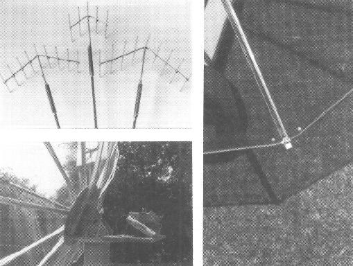
A simple dipole plus reflector feed antenna was designed, using the Numerical Electromagnetic Code software, to provide a ten dB illumination taper at the edge of the dish and a fifty-ohm terminating resistance. It was fabricated using 1-mm tinned copper wire. Assembly was facilitated by using a corrugated cardboard jig to hold the wires during soldering. The completed feed antenna was then attached to a length of solid coaxial cable terminated in a sleeve balun (see figure 6(c) and 7 for details).

The parabola and feed/preamp/receiver assembly was mounted on an altazimuth mount which was supported on a steerable trolley fitted with pneumatic tyres. This arrangement facilitated pointing of the telescope to any part of the sky. In practice, however, observations were confined to elevation angles above 30° to reduce pick up of thermal noise from the ground.

Figure 6. (a/left) The completed antenna and feed assembly on the altazimuth mount and trolley. (b/right) Hub assembly.

Figure 6. (c/top-left) Three feeds were used with the telescope. They are tuned to 1420.406, the H-line, 1665.405 MHz, the OH line, and 1537.825 MHz, the INMARSAT Pacific Ocean Satellite, the latter being useful for beamwidth determination and sensitivity checks for the antenna. (d/bottom-left) Rear view showing the scanning receiver, AC voltmeter and the prestressed truss technique used to make the ribs. (e/right> Method of fixing the aluminium fly-wire at the periphery of the dish using tubular aluminium struts, washers and pop rivets.

Figure 7. Design of the feed antenna for 1420.406 MHz. This design gives a feed point impedance of 50 ohms and also provides a 10 dB illumination taper at the dish edge to minimise spillover and noise pickup from the ground.

4 USING THE TELESCOPE

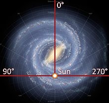
Observations were made along the galactic plane at galactic longitudes of 185° (that is towards the galactic anti-centre), 245°, and 330° under clear skies on 2 November 1991 between 2130 and 2400 AEST (1130 - 1200 UT). Additional observations of the Large and Small Magellanic clouds (LMC) and (SMC) were made under semi-overcast conditions on 5 November 1991 between 2145 and 2345 AEST (1145 - 1345 UT). Figure 8 illustrates all of the observing directions.

Two hydrogen line profiles were taken at each of these longitudes by taking serial measurements at programmed frequencies, nominally 50 kHz apart, and spanning the expected frequency range of the hydrogen line. For the Galaxy, this range was usually from 1420 to 1421 MHz. The Magellanic clouds were observed over a larger range, extending from 1419-1421 MHz.

Each measurement took approximately fifteen seconds, after which the result was read directly from the digital voltmeter and recorded. The scanner was then advanced to the next programmed channel and the process repeated. A complete profile containing around twenty measurements was completed in five minutes. The antenna was manually repositioned after each profile since no antenna drive was used.

Figure 8. A map of the galactic plane (after Kerr & Westerhout, 1964) showing the observing directions. Observations 1, 2 and 3 were made along the galactic equator. Observations 4 and 5 are of the Magellanic Clouds which are not in the galactic plane. At galactic longitude 245° (Puppis), two arms external to the Sun were observed. At galactic longitude 330° (Norma) observations were made tangentially to the spiral arms inside the Sun's orbit. At galactic longitude 185° observations were directed radially away from the galactic centre.

5 DATA ANALYSIS

Each raw profile was formed by averaging two 5-minute observation sets (figure 9). Linear detrending with respect to the baseline was sometimes necessary to eliminate temperature induced equipment drifts. The raw results were then corrected (ie frequency shifted) for the effect of solar motion with respect to the local standard of rest (LST), and the orbital motion of Earth around the Sun.

The LST correction is:

V_so = 18.38 cos b^ll cos (l^ll - 56.2^o) + 7.88 sin b^ll

The correction for the Earth's orbital motion about the Sun is:

V_eo = 29.8 cos θ

The effect of the Earth's rotation is small and has been neglected in these observations so that the total velocity correction is:

V_total = V_eo + V_so

Δf = - 1420.406 V_total / c MHz

Δf = - 4.7347 V_total kHz

The resulting corrected hydrogen line profiles are illustrated in figures 11 and 12.

Figure 9. The result of averaging two profiles at a galactic longitude of 245°. See section 6 for the interpretation of this profile.

6 RESULTS AND DISCUSSION

6.1 Galactic Observations

In the direction of galactic longitude 185°, we are observing towards the galactic anti-centre. The hydrogen line profile is therefore centred near the line rest frequency because the relative velocity between the LST and the atomic hydrogen in the arms under observation is close to zero. The profile, when observing at galactic longitude 245°, shows evidence of three separate peaks, probably representing the local arm (peak a) and two arms outside the local arm (peaks b & c) (figures 9 & 11). These peaks correspond to recession velocities of 55.2 km/s (b) and 86.9 km/s (c) respectively. No multi-peaked profile was observed at galactic longitude 330°, probably reflecting the fact that we are looking tangentially along several inner arms. These are apparently approaching rather than receding as in the previous observations.

Figure 10. Earth's orbital velocity (29.8 km/s) in its orbit around the sun contributes to the observed hydrogen line Doppler shift. This contribution can be calculated by resolving the velocity vector in the direction of the object under observation as shown above.

An interesting feature of observations inside the circle defining the orbit of the Sun around the galactic centre (figure 13) is that, when we observe along the line of sight, the maximum observed Doppler shift in the profile must originate from hydrogen emission at point A. In fact, a single measurement not only gives the orbital velocity at point A, but also the distance of A from the galactic centre. Assuming that the orbital velocity of point O (ie the LST) is 250 km/s, the equation in figure 13 can then be used to calculate the orbital velocity at A using the measured value of V_r (figure 11) which is 126 km/s. This calculation gives an orbital velocity V equal to 251 km/s. It is apparent that the orbital velocity at A, 5 kpc from the galactic centre and at position O at 10 kpc, are almost equal.

Figure 11. Corrected hydrogen line profiles for the observations at galactic longitudes of 185, 245 and 300 degrees (see section 6 for details). The galactic latitude was zero.

6.2 Magellanic Clouds

Figure 12 shows the results of the Magellanic Cloud observations. Interesting features of these observations are firstly, that the measured antenna temperatures were about the same (21 K) for each cloud, despite the fact that the LMC is visually brighter than the SMC, and secondly, the corrected Doppler were large, -280 km/s for the LMC and -147 km/s for the SMC. Considering the galactic longitude and distance of the clouds with respect to the Sun, these large recessional velocities must reflect the Sun's motion around the galactic centre rather than the recessional velocity of the clouds with respect to the galactic centre.

Figure 12. Corrected hydrogen line profiles for the Magellanic Clouds. Note the much lower line intensities compared with galactic observations in figure 10, and the large Doppler shifts, in excess of -1.5 MHz, indicating a large apparent velocity of recession of the clouds from the Sun (more correctly from the local standard of rest - LST).

Towards a Galactic Model

The galactic model which emerges from these preliminary observations is in agreement with the currently accepted picture of our galaxy, although further observations will clearly be necessary to fill in the whole picture. Spiral arm structure could be clearly identified outside the arm which contains the Sun. The fact that the orbital velocity of hydrogen as a function of the distance from the galactic centre appears to be approximately constant indicates that the spiral arms do not rotate as a solid disc or in Keplerian orbits such as in the solar system, but instead they slide past each other rather like athletes running around a more or less circular track, all at the same speed (figure 14).

Figure 13. Geometry and equation which refers to the observations at a galactic longitude of 330°. A single observation taken inside the Sun's orbit, of the maximum profile Doppler shift (figure 11) can give the distance of the emitting region at A, from the galactic centre C, and the orbital velocity V of that region about the galactic centre. V_r is obtained from the measured Doppler shift.

Figure 14. An analogy of galactic rotation. Runners a, b and c, which are analogous to the stars or hydrogen atoms which populate the arms of the galaxy, run around a circular track at constant speed (orbital veloctiy). Some time after the start, runner 'a' on the middle track falls behind runner 'b' on the inner track and moves ahead of runner 'c' on the outside track. This radial sliding motion also characterises the galactic rotation.

7 CONCLUSION

This preliminary work establishes the feasibility of doing some useful radio spectral line measurements at the hydrogen line frequency using relatively simple and inexpensive commercially available equipment. The equipment design and construction, observations, data collection, and analysis have been an enormously rewarding exercise which we would thoroughly recommend to any person or group who would like to know more about the shape of the galaxy which is our home in a vast and awesome universe.

8 ACKNOWLEDGEMENTS

We should like to acknowledge the help of Dr Jim Caswell of the CSIRO Division of Radiophysics who gave enthusiastic support, particularly in discussions about the local standard of rest corrections. We would also like to thank Dr Warwick Wilson of CSIRO and Professor Trevor Cole of the University of Sydney. Professor John Kraus of the Ohio State University Radio Observatory, one of the great pioneer explorers of the cosmos at radio wavelengths, has always been a great inspiration through his many books, and his personal encouragement. Special thanks to Judi, MW's wife, who, despite a protracted illness, has always supported these activities when she was able, and never seems to have been unduly perturbed by the large antenna structures which have periodically sprouted from our small back garden over the last twenty years or so.

9 BIBLIOGRAPHY

The following books are excellent general introductions to the history and radiophysics of the hydrogen line observations. Although some of them may be out of print, they should be obtainable through a library service.

J Pfeiffer, The Changing Universe, Victor Gollancz Ltd, London, 1956.

WT Sullivan III, Classics in Radio Astronomy, D Reidel Publishing Company, Dordrecht, Holland, 1982. [This book contains reprints and discussions about some ot the classic hydrogen line papers conveniently gathered in one place.]

T Page, L.W. Page editors, Stars and Clouds of the Milky Way - The Structure and Motion of our Galaxy, The Macmillan Company, New York [Part of the Macmillan Sky and Telescope Library of Astronomy.]

JD Kraus, Radio Astronomy 2nd edition, Cygnus-Quasar Books, Powell, Ohio 1986. [This book contains a considerable amount of other useful information about radio-astronomy and radio telescopes.]

J.D. Kraus, Our Cosmic Universe, Cygnus-Quasar Books, Powell, Ohio, 1980.

F Graham Smith, Radio Astronomy, Pelican Books, 1974.

RC Jennison, Introduction to Radio Astronomy, Newnes, London, 1966.

J.H. Piddington, Introduction to Radio Astronomy, Hutchison, 1961.

Kerr, FJ., and G. Westerhout, "Distribution of Hydrogen in the Galaxy", in: A. Blaauw and M. Schmidt (eds.), Galactic Structure, Vol. 5, Chap. 8, University of Chicago Press, Chicago, 1964.

Australian Space Academy

Home