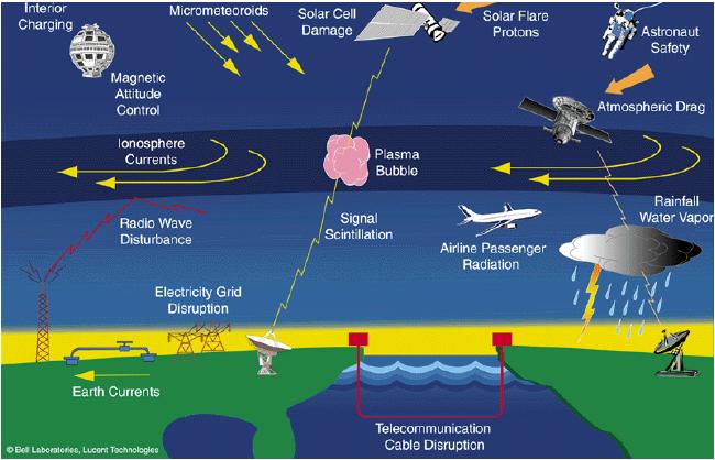
Originally drawn by Louis Lanzerrotti of Bell Labs, this now widespread figure shows some of many effects of space weather that can be traced back to solar, interplanetary and terrestrial domains.
THE SPACE WEATHER DOMAIN
Space weather covers several major domains. From the Sun (convection zone, photosphere, chromosphere and corona) where most of space weather originates, through the interplanetary medium to the Earth (magnetosphere, ionosphere, and surface) where the effects of space weather are felt. Each of these domains originates, transmits or receives a plethora of electromagnetic and particulate radiations of varying energies. And each type of radiation can result in a range of effects dependent upon the host sensitivity.
Each space weather source or effect can be measured and quantified by numbers or indices. More recently the development of simplified scales based on some of these numbers or indices has occurred, ostensibly to allow easier public understanding of space weather disturbances. So far the three scales adopted have been based on the negative effects of space weather. However, it is quite possible to produce scales that highlight the positive effects of space weather. These might more accurately be described as the background status of space weather. They are generally time averages over longer periods than the disturbance scales refer to and they thus indicate an average behaviour compared to a peak value of a short term disturbance.
Originally drawn by Louis Lanzerrotti of Bell Labs, this now widespread figure shows some of many effects of space weather that can be traced back to solar, interplanetary and terrestrial domains.
THE SOLAR DOMAIN
The Sun is the source of most, but not all, of the space weather effects we experience near the Earth. There are several manifestations of solar activity and these are all linked in some way to the solar magnetic fields which we believe originate at the base of the convection zone due to the differential rotation that occurs in the transition between the convection and radiation zones.
Sunspots are the most obvious manifestation of solar activity and historically the first to be observed, While we know that the Chinese were aware of sunspots for at least 2000 years (and probably also the Babylonians centuries before that), it was not until the first decade of the 1600’s that long term observations of sunspots were first started by Galileo. And it was not until 1843 that Heinrich Schwabe realised that the number of sunspots varied with an approximate 11 year period. In 1848 Rudolph Wolf produced the first sunspot index through the formula SSN = k ( 10 g + s ) where the sunspot number is a fraction k of ten times the number of sunspot groups plus the number of individual sunspots. The k value is to normalise observations from different observatories and different observers.
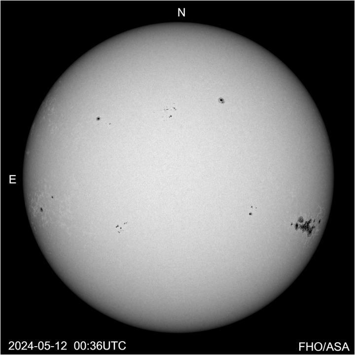
Telescopic image of the Sun (using a neutral density filter).
This shows sunspots clustered in groups and on each side of the solar rotational equator.
Credit: Mal Wilkinson
It is quite remarkable how this index (normally indicated by the letter R) has been found to relate to many geophysical effects on the Earth. However, we must realise that there are many different SSN indices relating to the integration time of this number. Rd is the daily index (usually averaged over a number of observatories), Rm is the monthly SSN, Ry is the yearly SSN, and RSSN is the smoothed SSN, a running average of 13 months given by RSSN = Σi=m-6 to m+6 Rmi . It is this last index RSSN that is used to drive many space weather models.
Drawing and counting sunspot groups ia an activity that has been carried out for centuries. However, the daily numbers obtained by different observers/observatories can be markedly dissimilar. We believe that the Central Limit Theorem comes strongly into play here such that when the strong double averaging of the smoother running SSN is reached we have a number that shows a Gaussian distribution and that thereby has a hope of meaning anything.
The Sun radiates across the electromagnetic spectrum although 99% of the power is concentrated in the IR and visible spectrum peaking at around 500nm (from a mean temperature of nearly 6000 K. Although this radiation from what astronomers call a G2 star does vary, the variation in total power is less than 1%. This is fortunate for humans as the average G2 star shows a variability of 4%. However at the EM spectral extremes the sun shows a variability of one million (six order of magnitude) in both the radio and X-ray regimes. It is this variability that creates two major aspects of space weather.
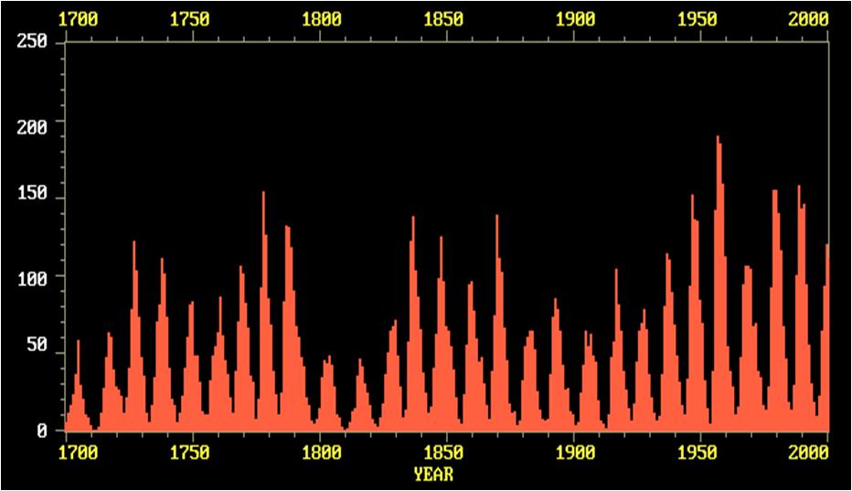
Plot of 300 years of the yearly or annual sunspot number.
NB: This is not the running smoothed SSN.
SOLAR INDICES
There are many physical parameters of the solar interior and the solar atmosphere that might be of interest but that cannot be easily measured. The accessible ones of interest for space weather are EM fluxes in the radio spectrum and the soft X-ray flux from 0.2 to 0.8 nm. In particular the 10.7 cm radio flux F10 is a useful index for overall solar activity. Other solar radio spectral frequencies effect various terrestrial systems and may be useful for specific operations (2). Radio flux/indices are stated in Solar Flux Units where 1 SFU=10-22 W/m-2/Hz.
Solar flares are high energy EM outbursts that can be viewed from the ground using narrow band filters (typically H-alpha). The first flare was seen in the visual continuum in 1859. These optical flares are categorised by a two part index nB where n=0,1,2,3,4 is the areal extent of the flare and B=0,F,N,B indicates the relative brightness of the flare (sub, faint, normal, bright). Although these indices are still used at ground solar observatories, space weather centres prefer to use the soft X-ray flux index of Class/Subclass (A0-A9, B1-B9, C1—C9, M1-M9 and X1-X28 where X28 is the extrapolated highest flare intensity so far observed (13 March 1989). The letter in this index relates to the power of ten of the X-ray flux in Wm-2 (A= 10-8 B=10-7 C=10-6 M=10-5 X=10-4) There is no corresponding areal extent given in the X-ray flare index.
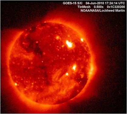
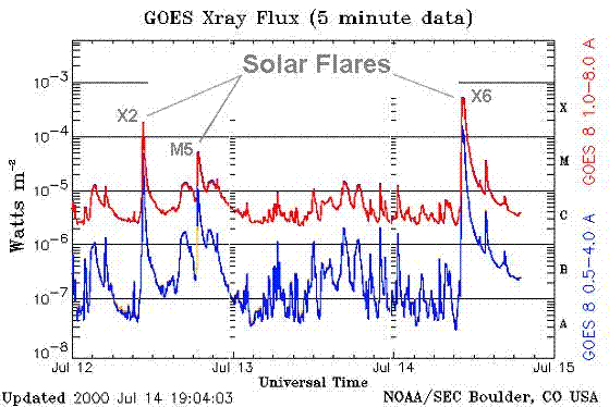
Solar X-ray image (top). Plot of full disc solar X-ray emission showing flares(bottom).
Although low and high energy ionised particles are ejected from the Sun they are not measurable from anywhere near the vicinity of the Sun, and they are also modified quite considerably by their passage through the interplanetary medium. Examples of such effects include the solar wind (which boils off from the million degree solar corona), coronal mass ejections (CME – large clouds of low energy particles ejected rapidly from the corona) and solar particle events (SPE/SEP – high energy [>1MeV] low mass [mostly protons with some alphas]) where the particle acceleration may occur in the solar atmosphere or IPM (InterPlanetary Medium).
R and F can be measured with ground equipment. On the other hand the X-ray and particle indices can only be measured from space and thus in the case of satellite failure, or in the event of space warfare (a likely scenario in the next decade) these indices will be denied to space weather centers. The more technically developed countries will suffer the most from satellite loss.
We feel that it is thus imperative to continue exploration of indices measurable from the ground and their relationship and correlation with indices measurable only from space.
THE INTERPLANETARY DOMAIN
The Sun radiates EM energy into the interplanetary medium. It also ejects particles into that medium. Both of these sources of energy travel through and are affected by the IPM to a lesser and greater extent dependent on their energy and nature. Because of the low density of particles in the IPM, EM energy is only subject to minor attenuation – except for very low frequency emissions. However frequencies up to a few hundred MHz from extrasolar sources may be subject to scintillation when passing through the IPM.
The solar wind may be regarded as an extension of the solar corona. It essentially boils off from the latter and travels through the IPM. Only the occasional measurement of the density, energy and flux of the solar wind is generally available away from the Earth. However the Space Weather Prediction Centre at Boulder has in the past provided speed and pressure parameters of the solar wind in the form of dials.

The solar wind speed is given in km/s. This can be used together with the dynamic pressure to estimate the particle flux. The IPM magnetic field is important because only at negative field does the wind couple into the magnetosphere.
THE COSMIC DOMAIN
Before we move to the terrestrial domain and its subdomains we need to consider the cosmic domain into the galaxy which is where galactic cosmic rays (GCR) originate. These very high energy particles penetrate to the Earth’s surface and below, although modified by the Earth’s atmosphere. This radiation is very significant for the expansion of the human presence into space, but must also be considered in terrestrial aviation. The US Federal Aviation Administration has developed a model (CARI) to predict this radiation, a model which uses a heliospheric potential index (stated in MV – megavolts). This index is derived from the shielding properties that solar magnetic fields, carried by the solar wind provide against the lower GCR energies.
THE MAGNETOSPHERIC DOMAIN
Without the solar wind the Earth’s magnetic field would look like that around a bar magnet. This field is generated by a conductive liquid moving around because of the Earth’s rotation. At mid-latitudes in Australia this has a surface value of ~50,000 nTesla. This field is modified by the solar wind and is compressed in the sunward direction and elongated in the antisolar direction.
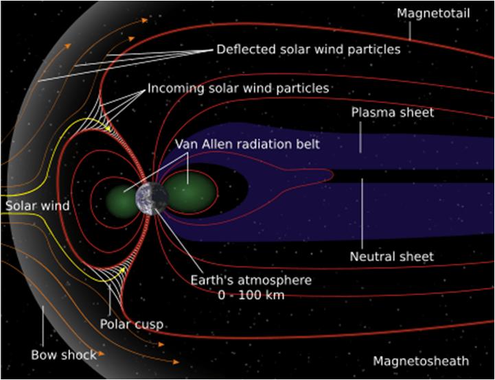
The Earth's magnetic field is compressed on the sunward side by the pressure of the solar wind. The magnetotail is comversely stretched out, dragged by the solar wind as it passes by the Earth.
The resulting ‘structure’, called the magnetosphere, is very complex domain and would require many indices to attempt to classify the diverse substructure. In fact the earliest attempts to characterise geomagnetic activity occurred in 1885 after it was found that this was linked to the earliest communication systems using wire.
Since then many indices have been developed to explain magnetic variations over different regions of the Earth. The ones that still remain and that are recognised are aa, Am, Kp, Dst, and AE. Most of these relate to a particular area of the Earth’s surface. Dst relates to the equatorial region and AE to the auroral areas.
The most used index in space weather is the Kp or planetary K-index. This is a unitless logarithmic index that goes from 0 to 9+ and is adjusted for latitude so that Kp = 9 (a major geomagnetic storm) corresponds to a magnetic variation of 400 nT at midlatitudes but 1500 nT at high latitudes.
THE IONOSPHERIC DOMAIN
In 1839 the polymath Gauss speculated that the upper atmosphere might contain ionised regions, and in 1878 Stewart suggested that a conductive layer in the atmosphere might explain geomagnetic disturbances . In 1901 Marconi used radio waves for transatlantic communication leading Kennelly and Heaviside to independently suggest that this over the horizon path was via the reflection of signals from an ionised layer in the upper atmosphere. It was not until 1924-5 that the existence and height of ionospheric layers was measured Appleton & Barnett (phase method) and Breit & Tuve (pulse).

The ionosphere is a complex structure with multiple peaks and valleys. The peaks are identified as layers. An overview graph of ionospheric electron density is shown above. Solar EUV (extreme UV) radiation is the main ionising source for the F-layer. Neutral atom collision remove most of the E and D layers at night. The F-layer is under magnetospheric control.
Ground based ionospheric radars can only elucidate ionospheric below the F layer peak. These features are specified by the indices foE, foF1, foF2, hmE, hmF1, hmF2 and others. However these only apply to one specific measurement. Various ionospheric models have been developed to produce these values given a solar index, time and date and location and geomagnetic index. This solar index might be considered a planetary ionospheric index. In Australia only, an ionospheric index has been developed from ionospheric data (the T index), although this is tied to a solar index RSSN for prediction .
With satellite nav/comm we need to consider the whole ionosphere and this is normally specified by the ionospheric Total Electron Content specified in TEC units where 1 TECU = 1016 electrons/m. Signal scintillation is also specified by the S4 index which goes from 0 to 0.5 (strong scintillation).
DISCUSSION - NUMBERS, INDICES and SCALES
The distinction between number, index and scale is mostly in the eye of the user. Index would normally be a simplification of the actual measured number relative to a specified unit. However, we have seen from the above that the two may be almost identical in many situations. In the current space weather context however, scales are most definitely unitless and cover a limited range of numbers. Five levels in particular allows for the easily understandable verbal levels of very low, low, medium, high and very high or shifted versions of these as applicable to the physical situation. The big problem with simple scales is to know what they represent. For a space weather effect that comes from the Sun but is modified severely according to season, time of day, location, etc it is very difficult to use a simple five level scale. However there are now 3 space weather scales developed by the US NOAA SWPC, and adopted by the World Meteorological organisation. There are also many space weather parameters that have not yet been addressed here eg meteoroid influx rate. There have also been developed several auroral indices/scales (4).
TERRESTRIAL WEATHER SCALES
The most important tropospheric parameters for humans are temperature and humidity . Wind speed and rain probability are probably next in line. The one parameter that has been given an index divorced from the measurement unit is wind speed. We have the logarithmic Beaufort scale (0 to 12) (mainly for mariners) and the cyclone category (1 to 5).
SPACE WEATHER SCALES - DISTURBANCE
The Space Weather Prediction Center at Boulder Colorado has developed 3 space weather scales to try and relate space weather to the general public. These are all disturbance scales and 2 derive from satellite measurements.
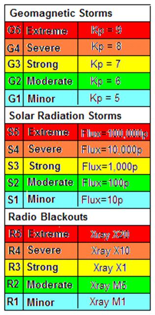
These scales cover three areas of space weather disturbances: geomagnetic storms, solar high energy particle events and solar X-ray flares. The geomagnetic scale is the only one directly related to a space weather index. The SPE scale is related to the solar particle flux above an energy of 10 MeV as measured at geosynchronous orbit, and the radio blackout scale is related to soft X-ray intensity (0.1 to 0.8 nm as measured at geosynchronous orbit). More complete detail on these five level scales is given at
SPACE WEATHER SCALES - BACKGROUND
The above scales give no indication of the background state of the space weather or of some of the positive effects that space weather may have. For instance, a high EUV flux will increase the frequency range available for high frequency communications, and a large geomagnetic index will intensify auroral displays and make them visible at lower latitudes. This may be more important to many members of the public than a minor power outage or loss of HF comms. An index to express the overall state of background solar activity. A high value of the F10.7 solar radio flux will indicate that space debris is likely to decay faster from low Earth orbits.
A simple solar background scale could be calculated from the formula:
REFERENCES
(1) O D Giersch, J Kennewell & M Lynch, “Solar Radiation Burst Statistics and Implications for Space Weather Effects”, Space Weather Journal v15 pp 1511-1522 (2017)
(2) Sean Eldridge, “The way we classify space weather needs to change”, Nature, v630 p270 (June 2024).
(3) P N Mayaud, “Derivation, Meaning, and Use of Geomagnetic Indices”, AGU Geophysical Monograph, (1980).
(4) < http://spaceacademy.net.au/env/terra/aurora/aurora.htm>
 Australian Space Academy