LOCATING GEOSYNCHRONOUS SATELLITES
INTRODUCTION
|
Geosynchronous satellites are those that appear to remain
nearly stationary in the sky as observed from a point on
the Earth's surface. They do so because their period of
revolution about the Earth is identical to the period
of rotation of the Earth about its polar axis.
A true geostationary satellite will remain absolutely fixed
at the same point in the sky as seen by a ground observer.
However, perturbing forces such as radiation pressure, Earth non-sphericity and lunar and solar gravitational forces, all
conspire to remove a satellite from a true geostationary
orbit. Ground directed manuevres are required to counteract
these forces and maintain the satellite in what is really
a geosynchronous orbit - an orbit that is close to but not
exactly geostationary. These corrections are termed station
keeping, and are carried out to keep the satellite in a
virtual box around the true geostationary point. This box
usually has dimensions of less than one degree of arc, as viewed from the ground. |
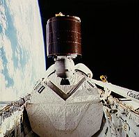
Australia's first geosynchronous satellite,
AUSSAT-A1 being deployed from the payload bay of Space Shuttle
mission STS-51I.
(NASA image) |
Station keeping has several
objectives. If the satellite is used to broadcast TV or data,
it means that small receiving antennae do not need to be moved
to track the satellite. It also helps minimise interference
between adjacent satellites using the same frequency band. And
it is one step toward minimising collisions between active
satellites.
Sometimes, if the station keeping fuel on board a geosat
becomes low, the inclination of the satellite (the angle that
its orbital plane makes with the Earth's equator) is allowed
to increase from zero. Such satellites show a figure of
eight motion in the sky. The satellite sweeps around the
figure of eight with a period of 24 hours.
Thus a ground observer is likely to see a combination of
secular drift, periodic motions (eg figure of eight) and
abrupt correctional changes (due to thruster firings) in
the motion of a geosynchronous satellite. However, these
are usually small, and for many locational purposes it is
adequate to compute look angles assuming the simplicity of
geostationarity.
SPECIFICATION OF A GEOSTATIONARY ORBIT
A geostationary orbit has specific orbital parameters. It is
first of all a circular orbit. This means that it has an
eccentricity of zero - its distance from the centre of the
Earth is always the same (42,165 km). It furthermore has an
orbital inclination of zero - its orbital plane is identical
to the Earth's equatorial plane. Lastly, it has a period
(related to its orbital radius) of 86164 seconds (about 23
hours 56 minutes 4 seconds), which is the time it takes the
Earth to rotate through 360 degrees.
The location of a satellite is usually computed using an
ephemeris program and a set of orbital elements. However,
for a stationary geosat, this is unnecessary and its position
may be computed using only geometry. The only parameter
needed to specify a geosat is its longitude. This is the same
as the longitude of a point on the Earth's equator directly
below the satellite itself.
Geosat longitude may be specified from 0 to 360 degrees,
measured eastward around the equator from the zero degree
meridian passing through Greenwich, England. Alternatively
it might be specified from 0 to +180 degrees (east) and
0 to -180 degrees (west). Note that +180 and -180 are the
same point.
GEOSAT GEOMETRY
We need both plane trigonometry and spherical trigonometry
to derive the equations needed to compute geostationary
satellite look angles.
We start with spherical trigonmetry. This will give us the
azimuth angle we require and also specify the plane in
which we use plane trigonometry to find the satellite
elevation.
Spherical geometry for geosat location.
The above diagram shows points on the surface of the Earth.
O is the observer, C is the centre of the Earth. P is a
point on the equator with the same longitude as the observer,
and T is the point directly below the satellite. All curved
lines on the diagram are parts of great circles.
We are interested in the spherical triangle OPT. The 'distance' t is the latitude of the observer, q is the
longitudinal difference between the observer and the satellite (or sub-satellite point), and g is the great circle
distance from the observer to the sub-satellite point.
The azimuth angle A is the angle measured from north of
the satellite, and this is the angle we are trying to
calculate.
The sides of the spherical triangle are related by:
Since we know the angles t and q, we can calculate the
angle g. Knowing this we can then calculate the azimuth
from the equation:
We then move to consider a plane triangle in the plane OTC
which contains both the observer and the satellite.
Plane geometry for geosat location
In the triangle COS, the satellite elevation is given by:
tan(e) = [(R+h)cos(g) - R] / [(R+h)sin(g)]
and the slant range to the satellite can be found from:
ρ = sqrt [ R2 + (R+h)2
- 2 R(R+h)cos(g) ]
To complete our calculations we need only to know that
R=6378 km and r=(R+h)= 42165 km, which are the equatorial
radius of the Earth and the satellite orbital radius
respectively.
These formula assume a perfectly spherical Earth, whereas it
is in fact an oblate spheroid with the polar radius less
than the above quoted equatorial radius. Calculations with
an oblate Earth model show that the errors incurred from the
spherical approximation amount to less than 0.1 degree in
azimuth and elevation and 10 km in slant range, at
mid-latitudes. This error is less than many station keeping
regimes.
GEOSAT LOOK ANGLE CHARTS
The above formula can be used to plot look angle charts.
These show both azimuth and elevation angles as a function
of observer latitude and longitudinal difference from the
satellite.
The chart below is the one to use at mid-latitudes.
The azimuth contours are shown in white or red and are
plotted every 2 degrees. The elevation contours are also
plotted every 2 degrees in blue or cyan. The chart can
thus be read to an accuracy of one degree with ease.
The azimuth angles shown in the above chart are in the range
from 0 to 90 degrees. The true azimuth is computed from
these values according to the quadrant in which the observer
lies with respect to the satellite. The modification
formulae are shown in the quadrant diagram below.
As an example, consider an observer at a latitude of 40
degrees north and 32 degrees to the east of the desired
satellite. From the look angle chart we find an elevation
of 34 degrees and an azimuth of 44 degrees. However, as the
observer is in the quadrant to the north-east of the satellite, the true azimuth is 180+44 or 224 degrees.
For observers in the tropics the look angle chart becomes very
congested, and an equatorial supplement is provided below.
Note that a geosynchronous satellite is below the horizon
when the great circle distance to its sub-point exceeds
81 degrees. This means no geosynchronous satellite coverage
in the polar regions. Geosat communication is possible
around the coastline of Antarctica but necessitates very
large ground antennae (eg 20 metre class dishes).
EQUATORIAL/POLAR COORDINATES
For astronomical and some other purposes, it is more
convenient to have the coordinates of a geosynchronous
satellite in terms of declination(δ) and hour angle(HA).
These may be computed from elevation and azimuth according to
the formula:
Note that δ is positive to the north of the equatorial
plane and negative to the south. The hour angle (HA) is
negative in the east and positive in the west.
The above two equatorial coordinates are constant because
the satellite is fixed in the sky. However, the stars are
not fixed and accurate positions are often derived from
stellar position comparison. For this purpose it is necessary
to change the hour angle coordinate into right ascension.
This is done using the formula:
where LST is the local sidereal time at the observing location.
Note that RA, LST and HA must all be in the same units, which
is usually hours, but may also be degrees. Note also that the
right ascension of a geosat is continuously changing, and if
this coordinate is specified it is vital to specify the time
of measurement.
The following plot shows how the declination of a satellite
changes with longitudinal difference.
The declination of a geosat will always lie between + and
- 9 degrees. For mid-latitudes the declination is around
-5 degrees in the northern hemisphere and +5 degrees in the
southern hemisphere. For a given location the declination of
any visible geosat never varies by more than about half a
degree.
The band in the sky across which geostationary
satellites are found is sometimes referred to as the Clarke
Belt, a tribute to the writer Arthur C Clarke who first
suggested the use of this orbit in 1945. The Clarke Belt is
shown for the Australian Space Academy site in the
diagram below. Several satellites are shown along the belt.
PROGRAMMING THE FORMULA
Coding the above formula into a computer program is
relatively straight forward. The main difficulty usually
arises in putting things in their correct quadrant.
A simple QBASIC program that produces geosat coordinates in
both the horizon coordinate system (elevation-azimuth) and
the equatorial coordinate system (declination-hour angle) is given below.
'GEOSATL.BAS
CLS
PRINT " GEOSTATIONARY SATELLITE LOOK ANGLES"
ER = 6378: HS = 35786!                    'earth radius / satellite ht
pi = 3.14159: dr = pi / 180               'pi /degrees to radians const
lon = 117: lat = -32                      'ground station long and lat (ASA)
ilon = CINT(lon)                          'round longitude to nearest integer
GT = lat * dr                             'convert ground lat to radians
form$ = "      ####.#      ##.#      ###.#   ##.###  ###.##    #####   #####"
PRINT USING "   Observer LAT=###.#  LON=####.# "; lat; lon
PRINT
PRINT "     SAT-LONG   ELEVANGLE  AZANGLE    HA      DEC     SLANT    GND"
PRINT "       (deg)      (deg)     (deg)    (hrs)   (deg)     (km)    (km)"
FOR SN = ilon - 85 TO ilon + 85 STEP 10  'only sats. within 81.3deg vis
  B = (lon - SN) * dr                    'longitude diff between sat & gnd
  GC = COS(B) * COS(GT)                  'GC is the great circle angle
  GC = ATN(SQR(1 - GC * GC) / GC)        'between gnd station and satellite
  IF GC < 1.419 THEN                     'if greater than 81.3deg skip
    gr = ER * GC                         'ground range to sat sub point
    az = ATN(TAN(B) / SIN(GT))           'compute azimuth angle
    IF GT >= 0 THEN az = az + pi         'adjust for northern hemisphere
    az = az - INT(az / 2 / pi) * 2 * pi  'ensure lies tween 0 and 360deg
    sr = SQR(ER ^ 2 + (ER + HS) ^ 2 - 2 * ER * (ER + HS) * COS(GC)) 'slant range to sat
    ZA = ((ER + HS) ^ 2 - sr ^ 2 - ER ^ 2) / 2 / ER / sr  'compute zenith angle
    ZA = ATN(SQR(ABS(1 - ZA * ZA)) / ZA): el = pi / 2 - ZA  'of satellite then elevation
    DC = COS(az) * COS(GT) * SIN(ZA) + SIN(GT) * COS(ZA) 'compute declination
    DC = ATN(DC / SQR(1 - DC * DC))                 'with simulated ASIN func
    HA = (COS(ZA) - SIN(GT) * SIN(DC)) / COS(GT) / COS(DC) 'compute hour angle of sat
    HA = ATN(SQR(1 - HA * HA) / HA)               'with simulated ACOS func
    IF az < pi THEN HA = -HA                      'take care of sign
    HA = HA / dr / 15
    S = SN + 180: S = S - INT(S / 360) * 360 - 180  'sat lon to lie -180 to 180
    PRINT USING form$; S; el / dr; az / dr; HA; DC / dr; sr; gr
  END IF
NEXT SN
END
A typical output is displayed below.
|
            GEOSTATIONARY SATELLITE LOOK ANGLES
              Observer LAT=-32.0  LON= 117.0

SAT-LONG  ELEVANGLE  AZANGLE    HA      DEC     SLANT    GND
 (deg)      (deg)     (deg)    (hrs)   (deg)     (km)    (km)
  42.0       4.0      278.1    5.487    4.70    41236    8607
  52.0      12.5      283.9    4.801    4.81    40320    7681
  62.0      21.0      290.4    4.098    4.91    39457    6779
  72.0      29.3      297.9    3.380    5.01    38678    5917
  82.0      37.1      307.1    2.647    5.10    38011    5120
  92.0      44.0      318.7    1.901    5.17    37485    4427
 102.0      49.3      333.2    1.145    5.22    37120    3896
 112.0      52.4      350.6    0.382    5.25    36934    3601
 122.0      52.4        9.4   -0.382    5.25    36934    3601
 132.0      49.3       26.8   -1.145    5.22    37120    3896
 142.0      44.0       41.3   -1.901    5.17    37485    4427
 152.0      37.1       52.9   -2.647    5.10    38011    5120
 162.0      29.3       62.1   -3.380    5.01    38678    5917
 172.0      21.0       69.6   -4.098    4.91    39457    6779
-178.0      12.5       76.1   -4.801    4.81    40320    7681
-168.0       4.0       81.9   -5.487    4.70    41236    8607
|
The last column in the above table is the great circle distance
from the observer to the satellite sub-point.
 Australian Space Academy