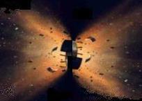
From a drawing by W Hartmann
INTRODUCTION
In articles on space debris and debris collisions, it is often stated that the average collision velocity between two objects in low Earth orbit (LEO) is around 10 kilometres per second. This should be contrasted with LEO orbital velocity which is around 7.5 km/s.
At first sight 10 km/s seems rather high. For a head-on collision, the maximum collision velocity is twice the orbital velocity, or 15 km/s. For a tail 'collision' the velocity is zero. One might assume that the average collision velocity is half way between these two, or 7.5 km/s. However, there are many more nearly head-on collisions than there are nearly tail-on collisions.
The situation is analogous to driving along a freeway. If you keep to the correct side of the road (left in Australia), you and all the other traffic are going at about the same speed, and there are very few collisions. However, if you are stupid enough to drive on the wrong side on the road, all the traffic is coming directly toward you, and a collision is very likely.
This note will discuss the value of the mean collisional velocity in low Earth orbit.
ORBITAL VELOCITIES
If we assume circular orbits (not a bad approximation for a large number of space objects in LEO) then the orbital velocity varies only as function of the height of the orbit. This can be calculated directly using Kepler's law, or derived from Newton's second law of motion and graviational force law. Values for selected heights covering most of the LEO range are given in the table below.
| h (km) | vo ( km/s ) |
| 300 | 7.73 |
| 500 | 7.62 |
| 700 | 7.51 |
| 900 | 7.40 |
| 1100 | 7.30 |
| 1300 | 7.21 |
h is the orbital height above the Earth's surface and vo is the orbital velocity (speed).
POPULATION ALTITUDE DISTRIBUTION
The following graph from the NASA Orbital Debris Program Office (ODPO) shows the altitude distribution of space objects in low Earth orbit.
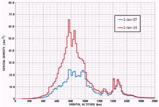
It can be seen that there is a large distribution of objects at around 800 km altitude, with a secondary peak around 1400 km. Collision probability is greatest where the population density is highest. At 800 km altitude, the orbital velocity is very close to 7.5 km/s, and we will use this velocity in subsequent calculations.
COLLISIONS
The diagram below shows two orbital objects with velocity vectors v1 and v2. Near the collision point these can be represented as straight lines making an angle θ between them. For a head-on collision θ = 180o (π radians), and θ is zero for a 'tail' collision.
The collision velocity vector vc is found by subtracting vector v2 from vector v1. This is accomplished geometrically by reversing the direction of v2 and laying it next to v1 as shown in the diagram. The resultant velocity vc is drawn from the tail of the first vector to the head of the second.
To calculate the magnitude of the collision velocity vc we use the cosine rule on triangle ABC:
COLLISION VELOCITIES
The graph below is a plot of the above formula for vc as a function of the collision angle θ.
Note that the collision velocity rises steeply as the collision angle increases from zero and then it flattens out as θ approaches a head-on collision.
If there is a random distribution of possible collision angles from 0 to 180 degrees, we might expect that the mean collision velocity occurs at an angle θ = 90o, and indeed it does, as shown in the following section. For a circular orbit at 700 km with an orbital velocity of 7.5 km/s this mean collisional velocity is 10.6 km/s.
MEAN COLLISION VELOCITY
The mean collision speed can be approximated by the formula:
The above solution was found by 'numerical integration'. We can also find an exact analytical solution by evaluating the integral
NON-UNIFORM POPULATIONS
The above results are for an ideal space object population where there is a random distribution of possible collision angles - which implies that each collision angle (or equal ranges of collision angle) have equally likely probability of occurring. This is not the situation in real life, where there are few objects with an inclination close to zero (at least in LEO). The following histogram shows the distribution of inclination for about 150 bright orbital space objects in low Earth orbit.
To calculate the mean collision speed in the case of non-uniform populations we must compute a weighted average. Such a computation by an Italian group (Rossi & Farinella, 1992) came up with a mean vc of 9.7 km/s - so our simple approach using the random approximation did not do so badly.
REFERENCES
A Rossi & P Farinella, Collision Rates and Impact Velocities for Bodies in Low Earth Orbit, ESA Journal, 16, 339-348, 01/1992.
 Australian Space Academy