THE IONOSPHERE
The ionosphere is what we term a weak plasma, as only one percent of the neutral atoms in the upper atmosphere are ionised. Traces of ionisation exist from about 80 km to 1000 km in altitude, with the peak ionisation occurring around an altitude of 300 km. The maximum ionisation can vary from about 1010 to 1013 electrons per cubic metre.
Ionospheric ionisation is controlled by extreme ultraviolet and soft x-ray flux emitted by the Sun. The lower regions of the ionosphere show almost exclusive solar control in that the ionisation at any time is proportional to some function of the solar zenith angle at each point.
The upper layers of the ionosphere are strongly influenced by the Earth's magnetosphere.
In quiet conditions the ionosphere is horizontally stratified, except for transitions at the solar terminator (sunrise and sunset) when layer tilts are found.
However, variations in solar x-ray output and changes in the geomagnetic field are reflected in disturbed ionospheric behaviour. Interactions between the ionospheric plasma and the neutral atmosphere principally determine recombination times and plasma movement due to winds and propagating waves.
PLASMA-ELECTROMAGNETIC INTERACTIONS
Two fundamental properties of a plasma, the plasma frequency and the refractive index, determine the interactions between a plasma and electromagnetic radiation.
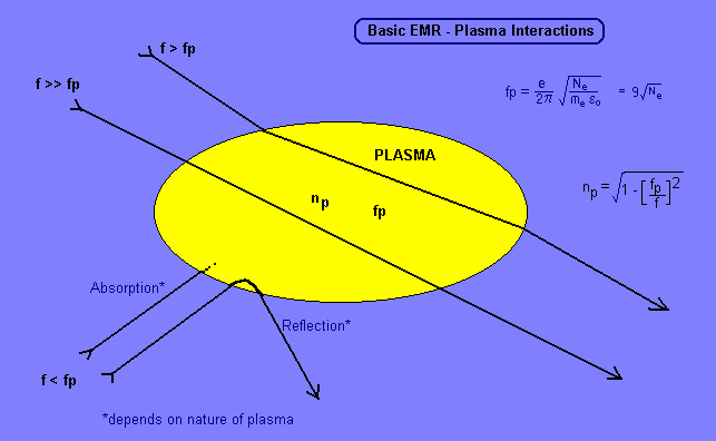
The plasma frequency, also called the critical frequency, is the frequency of oscillation that occurs in a plasma disturbed from local electrical neutrality as it relaxes back toward equilibrium. In essence, if we somehow cause a separation of positive and negative charge centres in the plasma (such a situation can occur after a shock wave passes through the plasma), then an electrostatic force will exist that will cause the electrons to travel back to the ions. They overshoot and the force reverses direction, creating a damped simple harmonic motion of the electrons about the ions. (The electrons do most of the moving as they are three orders of magnitude less massive than the ions). The frequency of this oscillation depends on basic fundamental constants of the electron together with the density of free electrons in the plasma.
In SI units the plasma frequency is nine times the square root of the electron density. A typically ionospheric maximum electron density of 1012 electrons per cubic metre thus gives us a plasma frequency of 9 MHz.
The refractive index of the plasma is dependent upon the plasma frequency and the radio frequency involved - and only on these two parameters.
Essentially the plasma appears opaque to EM waves below the critical frequency, and transparent to frequencies above. An EM wave where f<fp may be absorbed or reflected by the plasma depending upon the electron collision frequency with neutral atoms. A high collision frequency (lossy plasma) will result in absorption of the incident EM energy. A low collision frequency will allow the electrons to reradiate in phase producing what is in essence a reflection of the incident EM energy.
Above the plasma frequency, an EM wave will experience refraction (Snell's law) at each interface where the refractive index changes. Change may be abrupt or continuously varying.
The amount of refraction becomes progressively less as the EM frequency increases.
FORMATION OF THE IONOSPHERE
The diagram below illustrates the formation of an ionospheric layer. A specific wavelength in the solar radiation is absorbed by a specific molecular component in the upper atmosphere. Above an altitude of 100 km, the upper atmosphere is no longer homogenous (ie 20% O2 and 80% N2) but splits into different molecular and atomic components at different altitudes).
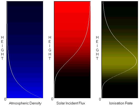
As the solar radiation propagates to lower atmospheric altitudes it encounters progressively more atmosphere which absorbs progressively more radiation, until there is no more of this wavelength to absorb. The process of absorption creates ionisation, which is balanced by recombination and at equilibrium a layer is formed with the general ionisation profile shown here. This profile is called a Chapman layer, after the geophysicist Sydney Chapman who derived the double exponential form of this profile:
where α is a loss (eg recombination) coefficient and z is a normalised height relative to the height of peak electron concentration Ne|max.
TYPICAL IONOSPHERIC DAYTIME PROFILE
A combination of several Chapman layers produces a good approximation to the actual ionospheric profile observed. The different ionospheric layers or regions are given the letter designators D, E, F1 and F2 as shown here. The first layer found was the E layer. Some stories say this represented the ionospheric layer of the Earth. Other stories say the letter E was assigned to allow for the labelling of lower layers if and when they were found. The lowest layer or region commonly referred to is the D region, although some researchers talk about a lower C layer created by galactic cosmic radiation.
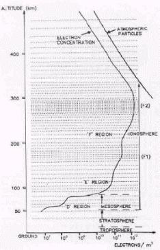
The D layer is highly absorptive due to the high collision frequency due to the relatively large neutral atmospheric density at this altitude.
The D, E and F1 layers recombine very quickly (within minutes) when the source of ionisation (the solar flux) is removed at sunset, and they thus disappear.
The F2 layer has a much lower recombination rate and persists during the night-time hours, being augmented by plasma blown around from the dayside by strong winds (several hundred km per hour) that exist at these altitudes.
IONOSPHERIC EFFECTS ON RADIO ASTRONOMY
The table below presents a list of ionospheric effects on various radio astronomical activities. They have been separated into effects of different order, both according to the magnitude of the effect and its possible significance to radio astronomy.
| FIRST ORDER EFFECT | |
| - Plasma opacity | |
| SECOND ORDER EFFECTS | |
| - Refraction | |
| - Dispersion | |
| - Faraday Rotation | |
| THIRD ORDER EFFECTS | |
| - Scintillations | |
| - Decoherence | |
| - Variable refraction | |
| - Phase stability | |
| FOURTH ORDER EFFECTS | |
| - Emission / Radiation |
Each of these effects will be discussed in more detail in following sections.
The first order effect is plasma opacity. Not many radio astronomy studies use these low frequencies but those that do are severely affected by this lower frequency limit.
Second order effects include refraction, dispersion (where signals of different frequencies experience different signal delays), and Faraday rotation (because the terrestrial ionospheric plasma exists in conjunction with the Earth's magnetic field).
Third order effects include signal scintillation (equivalent to stellar twinkling in optical astronomy), decoherence of a common signal over an extended baseline, and phase instability (where signal phases over an extended wavefront are varying).
The inclusion of a fourth order effect is unique to this presentation and is only added as a possible interference to EoR measurements. It is discussed later.
FIRST ORDER EFFECT
The first order effect is due to plasma opacity at frequencies below the plasma critical frequency. This is given by nine times the square root of the electron density. Maximum electron densities in the ionosphere typically range from 1010 to 1013 electrons per cubic metre.
The affected frequencies at the zenith of the radio telescope are equal to fc, which has a typical maximum value of 10 MHz at the Murchison Radio Observatory in central Western Australia (lat -27, lon 116). As the elevation of the observation decreases the affected frequencies increase to a maximum of about five times fc (or around 50 MHz at MRO).
It should be noted that the above discussion refers to a well behaved 'quiet' ionosphere. During certain seasons and at certain times, we find sporadic (in space and time) clouds or clumps of more highly ionised plasma forming. This is known as sporadic E (as it forms around 100 km, the altitude of the E-layer). This phenomenon can at times significantly alter affected frequencies, and of even greater significance, it can allow propagation of radio frequency interference into a radio quiet zone that one would not expect.
Radio astronomy fields affected by this first order effect include low frequency solar and interplanetary monitors (Note that the interplanetary medium has a plasma frequency of 50 kHz at Earth orbit (1 AU)). Studies of radiation from the plasma are obviously impossible from the Earth's surface. As these and higher frequencies (but well below fc) are suspected of being associated with the most dangerous space weather events we know (solar particle events), our inability to see them except via radiotelecopes in space is a big problem.
Jovian decametric radiation (5 to 40 MHz) can be severely affected by the first order effect.
And Epoch of Reionisation (EoR) studies may be affected if the EoR signal occurs for redshifts (z) of 30 or greater.
| Note: The EoR is expected to be found as a very small bump in the background emission in a plot of signal versus frequency. It is essentially a spectral line of the neutral hydrogen emission (which normally occurs at 1421 MHz in a rest situation) that has been redshifted to lower frequencies according to when in the evolution of the Universe it occurred. The frequency at which it will be shifted to is given by 1421/z where z is the redshift parameter. A red shift of z=30 will thus produce a line at around 50 MHz. |
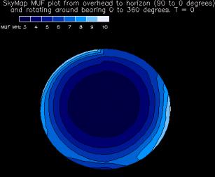
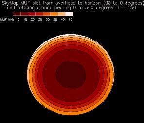
The two images below, courtesy of IPS Radio and Space Services, show the modelled sky transparency over the Murchison Radio Observatory for conditions of minimum (left) and maximum (right) expected ionospheric densities. The colour at any point on the sky indicates the frequency below which the ionosphere is opaque to radio signals. At any given geographic location, ionospheric density will vary with time of day, season, and solar EUV output. The latter shows a good average correlation to sunspot number.
|
|
SECOND ORDER EFFECTS - QUIET IONOSPHERE
Second order ionospheric effects are those effects that are always present, even during times when the ionosphere is quiet, or undisturbed due to transient space weather events.
Ionospheric refraction causes radio sources to appear in locations slighty different than their true sky position, and thus introduces a positional uncertainty in radio sky images. At moderate elevations the refraction is around one to two minutes of arc at 100 MHz, increasing at lower elevations.
A plasma is a dispersive medium. By this we mean that the time delay introduced in the propagation of a radio wave through a plasma varies with frequency, being less for higher frequencies. This delay is typically 1.5 microseconds at 100 MHz.
As we will shortly see, the ionospheric delay is only a very small fraction of the overall delay imparted to a signal propagating through the interstellar medium, for although the ISM has much lower electron densities than the ionosphere, the distances involved (thousands of parsecs) produce a much larger delay.
Faraday rotation is the rotation of the plane of polarisation of a linearly polarised signal passing through a plasma in a magnetic field. The ionosphere will typically rotate a signal three full rotations at 100 MHz.
THIRD ORDER EFFECTS - DISTURBED IONOSPHERE
First and second order effects exist at all times - that is they are effects due to the background or quiet ionosphere. However, when the ionosphere becomes disturbed, due to the impact of transient space weather events such as a geomagnetic storm, we then see third order effects.
Scintillations or 'twinkling' of radio sources cause image degradation. Strong scintillations can result in the signal dropping below the radiotelescope noise level, or alternatively receiver saturation for strong signals, causing non-linear effects and artefacts.
Variable refraction causes image distortion.
Phase instability causes positional changes and signal decorrelation in interferometers.
Decoherence may be introduced into Very Long Baseline Interferometry (VLBI).
Ionospheric disturbances producing the above effects are expected to be small and infrequent at Australian mid-latitude sites such as the Murchison Radio Observatory.
FOURTH ORDER EFFECTS
Fourth order effects are expected to be very small, and if they occur of significance only for EoR studies.
Essentially the ionosphere is a hot plasma (at around 1500 K kinetic temperature). Hot plasmas may radiate.
Possible mechanisms are through bremstrahlung and plasma radiation at the plasma frequency and its harmonics.
Any emission is undoubtedly very small, and we have not seen any papers to indicate any knowledge of such radiation.
However, such radiation may be significant as the EoR signal is expected to be a 25 milliKelvin change in a 250 Kelvin background! (ie four orders of magnitude below the background).
TYPICAL IONOSPHERIC CHANGES IN RADIO ASTRONOMY MEASURES
| Quantity | Typical value @ 100 MHz | Frequency dependence |
| Refraction | 1.5 arcminutes | 1/f2 |
| Polarisation | 10 radians | 1/f2 |
| Phase change | 1000 radians | 1/f |
| Path length | 500 metres | 1/f2 |
| Absorption | 0.01 dB | 1/f2 |
The above table summarises the typical second order ionospheric effects at a frequency of 100 MHz. Actual values encountered may vary by up to an order of magnitude each side of these 'typical' values.
Note that all effects except the phase change scale as the inverse frequency squared.
COLUMNAR ELECTRON DENSITY UNITS
The SI unit of columnar electron density is electrons per metre squared (often referred to as inverse metre squared - the number of electrons being a dimensionless quantity).
The ionospheric unit is the TECU or total electron content unit where:
The radio astronomical unit of TEC is called the DM (or dispersion measure) and is measured in parsecs per cubic centimetre! (or electrons per cubic centimetre per parsec).
The equivalence of the DM and TECU is given by:
The DM is a unit that is basically used by pulsar and other radio astronomers studying transient sources.
Typical DM's for pulsars range from 10's to 100's, and it can thus be seen that ionospheric plasma dispersion is quite insignificant. However, it is important in at least one radio astronomy experiment, as we will discuss later.
The ionospheric TEC ranges from about 1 to 100 TECU when looking through the ionosphere in a vertical direction. It may extend to 500 TECU for a low elevation slant path.
IONOSPHERIC TEC VARIATION
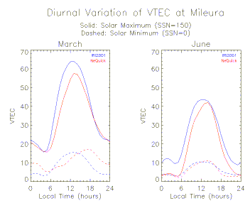
The graphs below show the modelled diurnal variation in ionospheric vertical total electron content for two different months and two different solar activities (low and high). The months chosen give minmum (June) and maximum (March) peak TEC values for a given value of solar EUV emission (of which we use sunspot number as a proxy). The location for these graphs is the Murchison Radio Observatory (MRO) in Western Australia.
The image below shows how the TEC varies at MRO with elevation angle (ie the STEC or Slant TEC). This STEC is modelled at high sunspot number (ie average maximal expected ionospheric density)
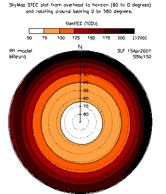
Both images above are courtesy of IPS Radio and Space Services.
ROTATION MEASURE UNITS
In radio astronomy Faraday rotation is specified by a 'Rotation Measure' which is a wavelength independent value with units of radians per square metre. The actual rotation experienced by an EM signal is thus the RM multiplied by the square of the signal wavelength.
As the ionosphere produces 10 radians rotation at 100 MHz (a typical value) or a wavelength of 3 metres, the ionospheric RM is typically 10 / 32 or about unity.
Most radio astronomy sources show much larger RM's than unity due to the very large interstellar distances involved.
SCINTILLATIONS IN RADIO ASTRONOMY
Ground-based radio astronomy observes three different scintillation sources:
| Region | Timescale | Critical Source Size |
| Ionosphere | 30 seconds | 10' |
| Interplanetary (IPM) | 1 second | 2" |
| Interstellar (ISM) & Intergalactic (IGM) | Days/Months | ? |
Ionospheric scintillations typically have periods greater than 10 seconds, whereas interplanetary scintillations have periods less then 10 seconds. A filter can thus be used to separate the two except when strong ionospheric scintillations cause non-linear mixing of the two signals.
Interstellar scintillations typically have very much longer timescales, and are due to refractive interference, although a fast diffractive type of interstellar scintillation is now known.
Sources have to be less than two arcseconds in angular diameter to show interplanetary scintillation, whereas they can be up to ten arcminutes across and still be affected by ionospheric scintillation.
The table refers to a frequency of 100 MHz. However, most interstellar scintillation is observed at frequencies in the GHz range.
IONOSPHERIC SCINTILLATION
One index of ionospheric scintillation is the S4 index, which is computed from the normalised variance of the scintillation power:
The graph below shows the (modelled) worst case expected for S4 (90th percentile) over Australia (courtesy IPS Radio and Space Services).
Equatorial scintillations are driven by (correlated with) solar EUV output, whereas auroral scintillations are driven by (correlated with) geomagnetic activity. The figure is drawn for maximum values of solar radiation and maximum geomagnetic activity. The geomagnetic activity would only exist at this level for a few hours.
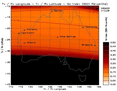
Even in this extreme case, the S4 value for the Murchison Radio Observatory is still less than 0.2. (S4 can range from 0 to 1.0). Weak scintillations are generally characterised by S4 values from 0 to 0.3."
EXTREME EXAMPLES OF IONOSPHERIC EFFECTS
Although the ionosphere adds negligible dispersion to pulsar signals (with typical pulse widths of several tens to several hundred milliseconds), there is one radio astronomy experiment in which the ionospheric TEC is significant. This is an experiment that Ron Ekers (CSIRO) and his group have been pursuing for several decades, and that is now known by the name LUNASKA. It is an attempt to use the Moon as a neutrino detector. Neutrinos hitting the lunar regolith are expected to produce very narrow pulses (eg 1 nanosecond). Such narrow pulses will show substantial dispersion due to passage through the ionosphere. An accurate knowledge of ionospheric TEC is required to de-disperse these pulses and render them detectable.
Most ionospheric effects scale with inverse frequency squared, and, with the possible exception of Faraday rotation, are negligible above 1 GHz. It is thus interesting to learn that in high accuracy VLBI (Very Long Baseline Interferometry), the ionosphere is the largest source of error (~1 cm) at 24 GHz!
EPOCH OF REIONISATION
Epoch of Reionisation experiments are looking for an extremely small spectral change (of the order of 25 milliKelvin) in a background sky temperature of hundreds to thousands of Kelvin (the latter if the EoR frequency is less than 100 MHz). All foreground sources (both natural and manmade) have to be subtracted from the signal to leave only the background signal.
We really don't know how the ionosphere will affect this measurement.
Will inhomogeneities across the sky be significant (for non-imaging experiments) or will the variations with time average out?
Even a very small emission/radiation from a hot ionospheric plasma may be important. Particularly plasma radiation over a band of frequency produced from around the peak of the F-layer (or sporadic E). Selectively amplified harmonics of this signal could produce a spectral bump say around 50 MHz (5th harmonic), which might be mistaken for the EoR signal.
IONOSPHERIC SUPPORT FOR RADIO ASTRONOMY
1 The development of a climatological database to support specific project planning
2 An archive database of TEC and S4 values to help in assessing data quality and help data reduction and analysis. Although this type of data is available in the automated calibration of interferometric images (it is often thrown away because of the data volume), quick look graphs from dedicated ionospheric sensors could provide a fast alert and/or confirmation service for times of degraded imagery.
3 Dedicated support for specific projects such as LUNASKA and high accuracy VLBI.
IPS Radio and Space Services , now a part of the Australian Bureau of Meteorology, has over 60 years experience in monitoring the ionosphere over Australia, and making predictions from both current and archived ionospheric data.
Dedicated instruments measuring ionospheric TEC and scintillations, located at the site of major radio astronomy facilities, are required to provide direct support to many radio astronomy projects.
 Australian Space Academy